Types of mathematical models. Classification of mathematical models depending on the model operator Classification and examples of mathematical models

A mathematical model is a simplification of a real situation and is an abstract, formally described object, the study of which is possible by various mathematical methods.

Consider classification of mathematical models.

Mathematical models are divided:

1. Depending on the nature of the displayed properties of the object:

· functional;

· structural.

Functional mathematical models are designed to display information, physical, time processes occurring in operating equipment, during the execution of technological processes, etc.

In this way, functional models- display the processes of functioning of the object. They usually have the form of a system of equations.

Structural models- can be in the form of matrices, graphs, lists of vectors and express the mutual arrangement of elements in space. These models are usually used in cases when the problems of structural synthesis can be posed and solved, abstracting from the physical processes in the object. They reflect the structural properties of the designed object.

A group of methods called schematic models - These are methods of analysis that include a graphical representation of the operation of the system. For example, routings, diagrams, multifunctional operation diagrams, and flowcharts.

2. By methods of obtaining functional mathematical models:

· theoretical;

· formal;

· empirical.

Theoretical get based on the study of physical laws. The structure of the equations and the parameters of the models have a certain physical interpretation.

Formal are obtained based on the manifestation of the properties of the modeled object in the external environment, i.e. considering the object as a cybernetic "black box".

The theoretical approach makes it possible to obtain models that are more universal, valid for wider ranges of variation of external parameters.

Formal - are more accurate at the point in the parameter space at which the measurements were made.

Empirical mathematical models are created as a result of experiments (studying the external manifestations of the properties of an object by measuring its parameters at the input and output) and processing their results by methods of mathematical statistics.

3. Depending on the linearity and nonlinearity of the equations:

· linear;

· nonlinear.

4. Depending on the set of the domain of definition and the values ​​of the variables of the model, there are:

· continuous

· discrete (domains of definition and values ​​are continuous);

· continuous-discrete (the domain of definition is continuous, and the range of values ​​is discrete). These patterns are sometimes referred to as quantized;

· discrete-continuous (the domain of definition is discrete, and the range of values ​​is continuous). These models are called discrete;

· digital (domains of definition and values ​​are discrete)

5. By the form of links between output, internal and external parameters:

· algorithmic;

· analytical;

· numerical.

Algorithmic are called models presented in the form of algorithms that describe a sequence of unambiguously interpreted operations performed to obtain the desired result.

Algorithmic mathematical models express the relationship between the output parameters and the input and internal parameters in the form of an algorithm.

Analytical mathematical models such a formalized description of an object (phenomenon, process) is called, which are explicit mathematical expressions of output parameters as functions of input and internal parameters.

Analytical modeling is based on an indirect description of the modeled object using a set of mathematical formulas. The language of analytical description contains the following main groups of semantic elements: criterion (criteria), unknowns, data, mathematical operations, constraints. The most essential characteristic of analytical models is that the model is not structurally similar to the modeling object. Structural similarity here is understood as the unambiguous correspondence of the elements and links of the model to the elements and links of the modeled object. Analytical models include models based on the apparatus of mathematical programming, correlation, and regression analysis. An analytical model is always a construct that can be analyzed and solved mathematically. So, if the apparatus of mathematical programming is used, then the model basically consists of an objective function and a system of constraints on variables. The objective function, as a rule, expresses the characteristic of an object (system) that needs to be calculated or optimized. In particular, it can be the productivity of the technological system. Variables express the technical characteristics of an object (system), including variable ones, restrictions are their permissible limit values.

Analytical models are an effective tool for solving the problems of optimizing the processes occurring in technological systems, as well as optimizing and calculating the characteristics of the technological systems themselves.

An important point is the dimension of a particular analytical model. Often, for real technological systems (automatic lines, flexible production systems), the dimension of their analytical models is so large that obtaining an optimal solution turns out to be very difficult from a computational point of view. In this case, various techniques are used to increase the computational efficiency. One of them is connected with splitting a problem of large dimension into subproblems of lower dimension so that autonomous solutions of subproblems in a certain sequence give a solution to the main problem. In this case, problems arise in organizing the interaction of subtasks, which are not always simple. Another technique involves reducing the accuracy of calculations, due to which it is possible to reduce the time for solving the problem.

The analytical model can be investigated by the following methods:

· analytical, when they strive to obtain in general form the dependences for the required characteristics;

· numerical, when they seek to obtain numerical results for specific initial data;

· qualitative, when, having solutions in an explicit form, one can find some properties of the solution (estimate the stability of the solution).

However, analytical modeling gives good results in the case of fairly simple systems. In the case of complex systems, either a significant simplification of the original model is required in order to study at least the general properties of the system. This allows you to obtain indicative results, and to determine more accurate estimates, use other methods, for example, simulation modeling.

Numerical model characterized by a dependence of this kind, which allows only solutions obtained by numerical methods for specific initial conditions and quantitative parameters of the models.

6. Depending on whether the equations of the model take into account the inertia of processes in the object or do not take into account:

· dynamic or inertial models(written in the form of differential or integro-differential equations or systems of equations) ;

· static or non-inertial models(written in the form of algebraic equations or systems of algebraic equations).

7. Depending on the presence or absence of uncertainties and the type of uncertainties, the models are:

· deterministic e (no uncertainties);

· stochastic (there are uncertainties in the form of random variables or processes described by statistical methods in the form of distribution laws or functionals, as well as numerical characteristics);

· fuzzy (to describe uncertainties, the apparatus of the theory of fuzzy sets is used);

· combined (both types of uncertainties are present).

In the general case, the form of a mathematical model depends not only on the nature of the real object, but also on the problems for the solution of which it is created, and the required accuracy of their solution.

The main types of models are shown in Figure 2.5.

Let's consider one more classification of mathematical models. This classification is based on the concept of controllability. We will divide all MM conditionally into four groups.1.Prediction models (computational models without control). They can be divided into static and dynamic The main purpose of these models: knowing the initial state and information about the behavior at the boundary, to predict the behavior of the system in time and space. Such models can also be stochastic. As a rule, forecasting models are described by algebraic, transcendental, differential, integral, integro-differential equations and inequalities. Examples are models of heat distribution, electric field, chemical kinetics, hydrodynamics, aerodynamics, etc. 2. Optimization models. These models can also be divided into static and dynamic. Static models are used at the design level of various technological systems. Dynamic - both at the design level and, mainly, for optimal control of various processes - technological, economic, etc. There are two directions in optimization problems. The first includes deterministic tasks... All input information in them is fully definable. The second direction relates to stochastic processes... In these problems, some parameters are random or contain an element of uncertainty. Many problems of optimization of automatic devices, for example, contain parameters in the form of random noise with some probabilistic characteristics. Methods for finding the extremum of a function of many variables with various constraints are often called methods of mathematical programming. Mathematical programming problems are one of the most important optimization problems. In mathematical programming, the following main sections are distinguished.· Linear programming ... The objective function is linear, and the set on which the extremum of the objective function is sought is given by a system of linear equalities and inequalities.· Non-linear programming ... The objective function is nonlinear and nonlinear constraints.· Convex programming ... The objective function is convex and a convex set on which the extremal problem is solved.· Quadratic programming ... The objective function is quadratic and the constraints are linear.· Multi-extreme tasks. Problems in which the objective function has several local extrema. Such tasks seem to be very problematic.· Integer programming. In such problems, integer conditions are imposed on variables.

Rice. 4.8. Classification of mathematical models

As a rule, the methods of classical analysis for finding the extremum of a function of several variables are inapplicable to problems of mathematical programming. Models of the theory of optimal control are one of the most important in optimization models. The mathematical theory of optimal control belongs to one of the theories that have important practical applications, mainly for optimal control of processes. There are three types of mathematical models of optimal control theory.· Discrete optimal control models. Traditionally, such models are called dynamic programming models, since the main method for solving such problems is the Bellman dynamic programming method.· Continuous models of optimal control of systems with lumped parameters (described by equations in ordinary derivatives).· Continuous models of optimal control of systems with distributed parameters (described by partial differential equations).3. Cybernetic models (game). Cybernetic models are used to analyze conflict situations. It is assumed that a dynamic process is determined by several actors, who have several control parameters at their disposal. A whole group of subjects with their own interests is associated with the cybernetic system. 4. Simulation modeling ... The types of models described above do not cover a large number of different situations, such that can be fully formalized. To study such processes, it is necessary to include a functioning "biological" link - a person - in the mathematical model. In such situations, simulation is used, as well as examination methods and information procedures.

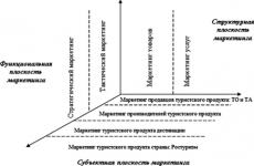
Mathematical models constitute an abstract part of the spectrum (Fig. 7.2), for the convenience of their use in various industries, including logistics, they are classified according to the six most representative features:

The method of obtaining the model;

The way of describing or representing an object or its properties;

The method of formalizing an object or its properties;

Membership at the hierarchical level;

The scale of the description of an object or its properties;

The degree of complexity of describing an object or its properties.

Bymethod of obtaining models are divided into theoretical , neural (perceptrons) and empirical .

Theoretical models are derived mathematically based on knowledge of the primary laws of classical mechanics, electrodynamics, chemistry, etc. Models obtained from real life on the basis of statistical processing of observation results form a group of empirical ones. The problem of constructing an empirical model includes the choice of the form of this model, suitable, as well as a reasonable degree of its complexity, compatible with the available experimental data.

In recent years, neural models (perceptrons) have become increasingly important in the field of modeling economic processes. The neural model (perceptron) consists of binary neural-like elements and has a simple topology.

The perceptron itself includes matrices of binary inputs (sensory neurons or retina, where input images are fed), a set of binary neural-like elements with fixed connections to subsets of the retina, a binary Neuro-like element with modified connections in these predicates (elements, decide).

Previously, the perceptron was used to solve the problem of automatic classification, in general, it consists in dividing the feature space between a given number of classes. In today's conditions, at the level of neural networks, it is possible to solve the problem of logistic forecasting, which is formalized through the problem of pattern recognition.

Consider the following example. There is data on the current demand for the company's products for six years (Ac = 6): 71, 80, 101, 84, 60, 73.

To formalize the task, we use the window method. Set the size of the windows η = 3, T= 1 and the level of excitation of the Neuro-like element s = 1. Next, using the method of windows with already fixed parameters n, t, s the following training sample is generated for the neural network:

As you can see, each subsequent vector is formed as a result of shifting the windows W and and W 0 to the right one element (s= 1). In this case, it is assumed that there are hidden dependencies in the time sequence as a set of observations.

The neural network, learning on these observations and adjusting its coefficients accordingly, tries to extract these patterns and form, as a result, the expected forecast function, that is, "build" model . Forecasting is carried out according to the same principle as the formation of a training sample.

By the way the object is described models are divided as follows:

1) algebraic;

2) regression-correlation;

3) probabilistic-statistical, combining models of the theory of queues, models of stocks and statistical models;

4) mathematical programming - linear programming, network (stream).

Regarding the first group of models - algebraic , it is necessary to immediately make a reservation that they, in essence, for the logistician are auxiliary in order to make the right decision. Algebraic models are commonly used in tasks such as tipping point analysis and cost-benefit analysis.

Regression-correlation models , representing the second group, is a generalization of extrapolation and statistical models and are used to describe the specifics of an object or its properties.

The third group consists of probabilistic statistical models , based on phenological phenomena and hypotheses. These models can be deterministic or stochastic. So, for example, the dependence V = φ (Χ), which is established according to the results of observations of random variables X and V the least squares method is a deterministic model. If we take into account the random deviations of the experimental points from the curve observed as a result of the experiments Y = φ (X) and write the dependence of B on X in the form B = φ (Χ)+ Ζ (where Ζ - some random variable), then we get a stochastic model in its ideal expression.

In this case, the quantities X and V can be both scalar and vector. Function φ (Χ) can be either a linear combination of these functions or a given nonlinear function, the parameters of which are determined by the least squares method.

Models linear programming are increasingly used to solve logistics problems.

Anyone who is familiar with mathematical programming knows that it is practically impossible to solve it in general form. However, the most developed in mathematical programming are linear programming problems.

In linear programming problems, the objective function is linear, and the constraint conditions include linear equalities and linear inequalities; variables may or may not be subject to the immutability requirement.

To demonstrate the simplicity of solving logistic problems using linear programming, we turn to two well-known problems:

The first is about the grandmother who is going to the market to sell the animals that have grown in her yard during the year;

The second is about nutrition.

The first task (about the grandmother)

The essence of this problem comes down to obtaining an answer to a simple question: "How much grandmother should be taken to sell live geese, ducks and chickens on the market so that it receives the greatest revenue, provided that it can deliver livestock weighing no more than R kg? ". In this case, the following are known:

Mass of chicken (t,), duck ( T 2 ) and goose (t3)

Cost of chicken (c7), duck (c2) and goose (c3).

Consider an algorithm for solving the problem.

1. To solve the problem, we denote the number, respectively, of chickens - X 1 ducks - X 2, geese - X 3 taken by the grandmother to sell to the market.

2. Let's compose the objective function of this task:

3. Let us describe the constraints on the solution of the problem.

The mass of goods, the grandmother can simultaneously deliver to the market, should not exceed R kilogram:

The value, and must be positive integers (), that is:

After completing the three described steps, we get a linear programming problem. Substituting the original values x, t, s and R, we find the answer to the question posed.

Second task (about nutrition)

Cafe "Bistro" buys food products from the store every day for preparing certain dishes for its visitors. The diet contains three different nutrients ( b) and need them, respectively, at least b 1, b 2, b 3 units. The store sells five types of different products X 1 - X 5 for the price, respectively S-I - s 5.

Each unit of the product i-th of the form ( X i) contains a and j units j-th nutrient, that is, for example, a 2 With shows that in units of the second product of the third nutrient there will be a 23 units.

Since the cafe operates surrounded by competitors, it is necessary to correctly determine the number of products of each type X 1 - x 5 worth buying. In this case, the following conditions must be met:

1) that the cost of products is minimal;

2) so that the diet contains all the necessary nutrients in the right amount.

The mathematical formulation of the solution to the problem will be as follows:

1. The objective function of this task is to minimize the cost of products X 1 - X 5. Mathematically, it will look like this:

2. Conditions for limiting the solution of the problem:

a) the amount of the first nutrient must be at least b 1 ,:

b) the amount of the second nutrient must be at least b 2 :

c) the amount of the third nutrient must be at least b 3:

It should be borne in mind that the number of products cannot have a negative number, that is:

For a correct understanding of the solution to the given problem, consider the following example.

Let in this problem we have the following initial data:

The objective function will look like this:

The minimum value of the function must be determined subject to the following restrictions:

Bearing in mind that the number of products cannot be negative, we assume that

As a result of solving the problem according to the presented initial data, we have the following answer: and. With these values, the objective function will have the following meaning:

Network (stream) models.

An important class of mathematical programming problems are the so-called network (flow) problems, in terms of which linear programming problems can be formulated.

Let us consider as an example the so-called transport problem (Fig. 7.3), which is one of the first flow problems, which was solved in 1941 by F.L. Hitchcock.

Suppose there are two factories (1 and 2) and three trains (A, B, C). The factories produce s1 and s2 units, respectively. Warehouses have the ability to store d1, d2 and d3 units of products, that is:

The challenge is to minimize the cost of transporting products from manufacturing plants to warehouses. Let's set the following initial conditions. Let's pretend that X ij - volume of products to be transported from i-th plant on j-th compound; с - - the cost of transportation of a unit of production with i-th plant on j-th compound. Then the objective function of the problem, the cost of transportation, will have the following form:

Rice. 7.3.

The condition that all products will be transported from each plant:

Equality data can be written in short form, namely:

The condition for filling the warehouses is as follows: moreover

This model can be described using a network, if we assume that the nodes of the network are factories and warehouses, and the arcs are roads for the transportation of goods (Fig. 7.3). The formulated transport problem is a special case of the problem of finding the minimum cost flow within the network.

Network tasks are used in the design and improved large and complex systems, as well as in the search for ways of their most rational use. First of all, this is due to the fact that with the help of networks it is quite simple to build a model of the system. The latter is based on the idea of ​​a critical path (CPM method) and assessment and observation tools (for example, the PERT-Program Evalution Research Task system).

In addition, networks allow you to:

Formalization of a model of a complex system as a set of simple systems (in this case, a logistics system as a set of its subsystems and links - procurement, warehouses, transportation, stocks, production, distribution and sales);

Drawing up formal procedures to determine the quality characteristics of the system;

Determination of the mechanism of interaction between the components of the control system in order to describe the latter in terms of its main characteristics;

Determination of the data required for the study of the logistics system and its main subsystems;

Initial investigation of the control system, drawing up a preliminary schedule for the operation of its components.

The main advantage of the network approach is that it can be successfully applied to virtually any problem where a network model can be accurately constructed.

A generalized characteristic of mathematical models classified according to the method of object description is given in table. 7.3. The table shows the most suitable areas of application of these models with a preliminary indicated accuracy of the estimates obtained. This information is useful for logisticians at the stage of building models or choosing the latter to solve a problem.

By the nature of the displayed properties of the object models are classified into structural and functional, which together reflect the relationship and mutual influence of individual elements on the processes occurring in the object during its operation or manufacture.

Structural models are intended to display the structural properties of the composition object, the relationship and relative position, as well as the shape of the components.

Functional models are intended to a greater extent for displaying the processes occurring in an object during its operation or manufacture, and, as a rule, contain algorithms that link phase variables, internal, external or output parameters.

Table 7.3

Characteristic features of mathematical models

By the way the object is formalized with the complexity of existing situations, it becomes necessary to simplify their description using analytical and algorithmic models, properly

"Abstracts" selected "essential" properties of objects and situations. Computer simulation of real objects is a valuable tool for analyzing complex service systems, service policies and investment choices.

The distribution of objects into hierarchical levels leads to certain levels of modeling, the hierarchy of which is determined by both the complexity of the objects and the ability of the controls. Therefore, according to belonging to the hierarchical level, mathematical models are divided into micro-, macro- and metamodels. The difference between these models lies in the fact that at a higher level of the hierarchy, the components of the model take the form of rather complex collections of elements of the previous level. The same qualities determine the division of models by the degree of scale and complexity of the description of the object.

The above classification of models is designed to help logisticians in more efficient and correct decision-making in order to implement the mission of the organization.

It was noted above that any mathematical model can be considered as some operator A, which is an algorithm or is determined by a set of equations - algebraic, ordinary differential equations (ODE), systems of ODE (SODE), partial differential equations (PDE), integro-differential equations (IDE), etc. (Fig. 1.6).

If the operator provides a linear dependence of the output parameters on the values ​​of the input parameters X, then the mathematical model is called linear( rice. 1.7). Linear models are easier to analyze. For example, the linearity property implies the superposition property of solutions, i.e. if the solutions for and for are known, then the solution for the output parameters for there is ... The limiting values ​​for linear models are achieved, as a rule, at the boundaries of the areas of admissible values ​​of the input parameters.

Linear behavior is inherent in relatively simple objects. Systems, as a rule, exhibit nonlinear multivariate behavior (Figure 1.8). Accordingly, the models are subdivided into non-linear ones.

Depending on the type of operator, mathematical models can be divided into simple and complex.

In the case when the model operator is an algebraic expression reflecting the functional dependence of the output parameters fot of the input X, the model will be called simple.

As examples of simple models, one can cite many laws of physics (universal gravity, Ohm's law, Hooke's law, Amonton-Coulomb's law of friction), as well as all empirical ones, i.e. obtained from experience, algebraic relationships between input and output parameters.

The model, which includes systems of differential and integral relations, can no longer be classified as simple, since for its research it requires the use of rather complex mathematical methods. However, in two cases it can be reduced to simple ones:

if the system of mathematical relations obtained for a similar model can be solved analytically;

if the results of computational experiments with a complex model are approximated by some algebraic dependence. At present, a fairly large number of approaches and approximation methods are known (for example, the least squares method or the method of planning experiments).

In practice, situations often arise when a satisfactory description of the properties and behavior of the object of modeling (as a rule, a complex system) cannot be performed using mathematical relations. However, in most cases it is possible to construct some kind of simulator of the behavior and properties of such an object using an algorithm that can be considered a model operator.

For example, if, as a result of observing an object, a correspondence table is obtained between the input X and the output values ​​of the parameters, then define the operator A, allowing you to get an "exit" for a given "input" is often easier using an algorithm.

Classification of mathematical models depending on the parameters of the model(fig. 1.9)

In the general case, the parameters describing the state and behavior of the modeling object are divided into a number of disjoint subsets

a set of input (controlled) influences on the object ();

a set of environmental influences (uncontrollable) ();

a set of internal (intrinsic) parameters of an object ();

set of output characteristics ().

For example, when modeling the motion of a material point in the field of gravity forces, the initial position and the initial velocity of the point at the moment of time can be the input parameters. Resistance and gravity characterize the impact of the external environment. The point mass is an intrinsic parameter. Point coordinate and speed (at) are output parameters. The assignment of parameters to input or output depends on the formulation of a specific problem. Therefore, there are always direct and inverse problems.

Input parameters, parameters describing the impact of the external environment, and internal (intrinsic) characteristics of an object are usually referred to as independent (exogenous) quantities. Output parameters are dependent (endogenous) values. In the general case, the model operator transforms exogenous parameters into endogenous .

By their nature, the characteristics of an object can be as follows quality and quantitative... For a quantitative characteristic, numbers are introduced that express the relationship between this parameter and the standard (for example, "meter"). In addition, the quantitative values ​​of the parameter can be expressed discrete or continuous quantities. Qualitative characteristics are found, for example, by the method of expert assessments. Depending on the type of the used sets of parameters, the models can be subdivided into qualitative and quantitative, discrete and continuous, as well as mixed.

When constructing a model, the following options for describing the uncertainty of parameters are possible:

deterministic- the values ​​of all parameters of the model are determined by deterministic values ​​(i.e., each parameter corresponds to a specific integer, real or complex number, or the corresponding function). This method corresponds to the complete certainty of the parameters;

stochastic- the values ​​of all or individual parameters of the model are determined by random variables given by the probability densities. For example, cases of normal (Gaussian) and exponential distribution of random variables;

accidental- the values ​​of all or individual parameters of the model are set by random variables, given by estimates of the probability densities obtained as a result of processing a limited experimental sample of these parameters;

interval- the values ​​of all or individual parameters of the model are described by interval values ​​specified by the interval formed by the minimum and maximum possible values ​​of the parameter;

fuzzy- the values ​​of all or individual parameters of the model are described by the membership functions of the corresponding fuzzy set. This form is used when information about the parameters of the model is set by an expert in natural language, and, therefore, in “fuzzy” terms such as “much more than five”, “near zero”.

Splitting models into one-dimensional, two-dimensional and three-dimensional applicable for such models, the parameters of which include the coordinates of the space, and is associated with the peculiarities of the implementation of these models, as well as with a sharp increase in their complexity with increasing dimension.

Like coordinates, time is an independent variable that can affect the rest of the model. Usually, the smaller the scale of the object, the more significant the dependence of its parameters on time.

Any object seeks to move into some equilibrium state, both with its environment and between individual elements of the object itself. Violation of this balance leads to changes in various parameters of the object and its transition to a new equilibrium state.

When constructing a model, it is important to compare the time of significant changes in external influences and the characteristic time transitions of the object to a new equilibrium state with the environment, as well as the relaxation time, which determines the establishment of equilibrium between individual elements inside the object. If the rate of change of external influences on the object of modeling is significantly less than the rate of relaxation, then the explicit dependence on time in the model can be neglected. In this case, they talk about quasi-static process.

The set of values ​​of the model parameters at some point in time or at this stage is called the state of the object.

If the rates of change of external influences and parameters of the state of the object under study are sufficiently high (in comparison with the rates of relaxation), then taking into account the time is necessary. In this case, the object of research is considered within the framework dynamic process.

If external influences remain constant or their fluctuations have little effect on the state of the object for a sufficiently long period of time, then at each fixed point of the investigated space the values ​​of the model parameters do not depend on time. For example, the velocity field of liquid particles in a long pipe in a laminar regime. Such processes are called stationary... As a rule, stationary models are used to describe various flows (liquid, gas, heat) in the case of constant conditions at the inlet and outlet of the stream. For such processes, time can be excluded from the number of independent variables.

If it is necessary to use time (or its analogue) as one of the essential independent variables of the model, then the model is called non-stationary... An example of a non-stationary model is a model of fluid movement in a pipe, but flowing out of a certain vessel.

Classification of mathematical models depending on the goals of modeling (Fig. 1.11)

The purpose descriptive models is the establishment of the laws of change in the parameters of the model. The resulting model describes the dependence of the output parameters on the input ones. Therefore, descriptive models are the implementation of descriptive and explanatory meaningful models at the formal level of modeling.

Optimization models are designed to determine the optimal (best) parameters of the simulated object from the point of view of a certain criterion, or to find the optimal (best) control mode for a certain process. Some of the model parameters are related to control parameters, changing which you can get various options for sets of values ​​of the output parameters. Typically, these models are built using one or more descriptive models and include some criterion that allows you to compare different options for sets of values ​​of the output parameters with each other in order to choose the best one. Constraints in the form of equalities and inequalities related to the features of the object or process under consideration can be imposed on the range of values ​​of the input parameters. The purpose of the optimization models is to find such admissible control parameters for which the selection criterion reaches its "best value".

Management models are used to make effective management decisions in various areas of purposeful human activity. In the general case, decision-making is a process comparable in complexity to the process of thinking in general. However, in practice, decision-making is usually understood as the choice of some alternatives from a given set of them, and the general decision-making process is represented as a sequence of such choices of alternatives.

The complexity of the problem lies in the presence of uncertainty both in terms of initial information and the nature of the impact of external conditions, and in terms of goals. Therefore, in contrast to optimization models, where the selection criterion is considered definite and the desired solution is established from the conditions of its extremality (maximum or minimum), it is necessary to introduce specific optimality criteria in management models, which allow comparing alternatives with various uncertainties of the problem.

Since the optimality of the decision made even in the same situation can be understood in different ways, the form of the optimality criterion in management models is not fixed in advance. This is the main feature of these models.

Classification of mathematical models depending on the implementation methods (Fig. 1.12)

The model implementation method is referred to analytical if it allows you to get the output parameters in the form of analytical expressions , those. expressions that use no more than a countable set of arithmetic operations and limit transitions. Examples of analytical expressions:

,

A special case of analytical expressions are algebraic expressions, in which a finite or countable number of arithmetic operations, operations of raising to an integer power and extraction of a root are used. An example of algebraic expressions: .

Very often, an analytical solution for a model is presented in elementary or special functions. To obtain the values ​​of these functions for specific values ​​of the input parameters, use their expansion in series (for example, Taylor). So, the exponential function can be represented by the following series:

Taking into account the different number of members of the series, it is possible to calculate the value of the function with varying degrees of accuracy. Thus, the value of the function for each value of the argument in this case is determined approximately. Models using this technique are called close.

Analytical methods for implementing the model are more valuable, but they are not always obtainable.

At numerical approach, the set of mathematical relations of the model is replaced by a finite-dimensional analogue. This is most often achieved by discretizing the original relations, i.e. passing from functions of a continuous argument to functions of a discrete argument. After discretizing the original problem, a computational algorithm is constructed. The found solution to the discrete problem is taken as an approximate solution to the original mathematical problem. The main requirement for a computational algorithm is the need to obtain a solution to the original problem with a given accuracy in a finite number of steps.

At imitation approach, the object of research itself is broken down into individual elements. In this case, the system of mathematical relations for the object-system as a whole is not written down, but is replaced by some algorithm that simulates its behavior and takes into account the interaction of models of individual elements of the system with each other. Models of individual elements can be both analytical and algebraic.

STAGES OF BUILDING A MATHEMATICAL MODEL

A distinctive feature of the mathematical models being created at present is their complexity, associated with the complexity of the objects being modeled. This leads to the complication of the model and the need for the joint use of several theories (often from different fields of knowledge), the use of modern computational methods and computer technology to obtain and analyze the simulation results. Today, the widespread use of models in the practice of engineering and technical activities has caused the need for an algorithm for constructing a mat. models.

The process of building any mathematical model can be represented by a sequence of stages shown in Fig. 2.1.

2.1. INSPECTION OF THE SIMULATION OBJECT

Mathematical models, especially those using numerical methods and computing technology, require significant intellectual, financial and time expenditures for their construction. Therefore, the decision to develop a new model is made only if there are no other, simpler ways to solve the problems that have arisen (for example, modifying one of the existing models). If this decision is nevertheless made, then the procedure is as follows.

The main purpose stage of the survey of the modeling object is the preparation of a meaningful formulation of the modeling problem.

The list of the main questions of interest about the object of modeling, formulated in a meaningful (verbal) form, constitutes a meaningful formulation of the modeling problem.

The survey stage includes the following work:

a thorough examination of the actual object of modeling in order to identify the main factors, mechanisms that affect its behavior, determine the appropriate parameters that allow describing the modeled object;

collection and verification of available experimental data on analogue objects, carrying out additional experiments, if necessary;

analytical review of literary sources, analysis and comparison of previously constructed models of this object (or similar to the object under consideration);

analysis and generalization of all the accumulated material, development of a general plan for the creation of a mathematical model.

All the material collected as a result of the survey about the knowledge about the object accumulated up to this point, the meaningful formulation of the modeling problem, additional requirements for the implementation of the model and the presentation of the results are drawn up in the form technical specifications for the design and development of the model.

Develop a mathematical model to describe the flight of a basketball thrown by a player into a basketball basket.

The model should allow:

calculate the position of the ball at any time;

to determine the accuracy of the ball hitting the basket after the throw with different initial parameters.

Initial data:

ball mass and radius;

initial coordinates, initial speed and angle of the ball throw;

center coordinates and radius of the basket.

2.2. CONCEPT FORMULATION OF THE MODELING PROBLEM

Conceptual formulation of the modeling problem- this is a list of the main questions of interest, formulated in terms of specific disciplines (physics, chemistry, biology, etc.), as well as a set of hypotheses regarding the properties and behavior of the object of modeling.

A conceptual model is constructed as some idealized model of an object, written in terms of specific disciplines. For this, a set of hypotheses is formulated about the behavior of an object, its interaction with the environment, and changes in internal parameters. As a rule, these hypotheses are plausible, since some theoretical arguments can be presented to substantiate them and experimental data based on previously collected information about the object can be used. According to the accepted hypotheses, a set of parameters describing the state of an object is determined, as well as a list of laws governing the change and relationship of these parameters with each other.

Example. Conceptual formulation of the problem of a basketball player.

The movement of a basketball can be described in accordance with the laws of classical Newtonian mechanics (Fig. 2.2).

Let's accept the following hypotheses:

the object of modeling is a basketball with a radius;

motion occurs in the field of gravity with a constant acceleration of gravity and is described by the equations of classical Newtonian mechanics;

the movement of the ball occurs in one plane perpendicular to the surface of the Earth and passing through the point of throw and the center of the basket;

we neglect the air resistance and perturbations caused by the ball's own rotation around the center of mass.

In accordance with the stated hypotheses, the coordinates and speed (its projections and ) the center of mass of the ball. Then, to determine the position of the ball at any moment of time, it is sufficient to find the law of motion of the center of mass of the ball, i.e. coordinate dependence and the projections of the velocity vector and the center of the ball from time to time. As an estimate of the accuracy of the throw, one can consider the horizontal distance (along the axis) from the center of the basket to the center of the ball at the moment when the latter crosses the horizontal plane passing through the plane of the basket ring.

Taking into account the above, we can formulate the conceptual formulation of the problem about a basketball player in the following form: determine the law of motion of a material point with a mass under the action of gravity, if the initial coordinates of the point are known , its initial velocity and angle of throw. The center of the basket has coordinates . Calculate the accuracy of the throw , where is determined from the conditions: , , .

Let us consider the features of the example of the conceptual formulation of the problem of a basketball player.

The first of the listed hypotheses is especially important, since it identifies the object of modeling. In this case, the object can be considered simple. However, the "player - ball - ring" system can be considered as an object of modeling. The model required to describe such a system will be much more complicated, since the player, in turn, represents a complex biomechanical system and its modeling is a difficult task. In this situation, the choice of only the ball as the object of modeling is justified, since it is its movement that needs to be investigated, and the player's influence can be taken into account quite simply through the initial parameters of the throw.

The hypothesis that the ball can be considered a material point is widely used to study the movements of bodies in mechanics. In the case under consideration, it is justified due to the symmetry of the shape of the ball and the smallness of its radius in comparison with the characteristic distances of movement of the ball. It is assumed that the latter is a ball with the same wall thickness.

The hypothesis of the applicability in this case of the laws of classical mechanics can be substantiated by the enormous experimental material associated with the study of the motion of bodies near the surface of the Earth with velocities much less than the speed of light. Considering that the height of the ball lies within 5-10 m, and the range is 5-20 m, the assumption of the constancy of the acceleration of gravity also seems reasonable. If the motion of a ballistic missile were simulated at a range and flight altitude of more than 100 km, then it would be necessary to take into account the change in the acceleration of gravity depending on the altitude and latitude of the place.

The hypothesis about the motion of the ball in a plane perpendicular to the Earth's surface limits the class of trajectories under consideration and greatly simplifies the model. The trajectory of the ball may not lie in the same plane if, during the throw, it is strongly twisted around the vertical axis. In this case, the speeds of points on the surface of the ball relative to the air on different sides of the ball will be different. For points moving against the stream, the relative speed is higher, and for points on the opposite side, moving along the stream, it is lower than the speed of the ball's center of mass. According to Bernoulli's law, the gas pressure on the surface is greater where its relative velocity is lower. Therefore, for the situation shown in Fig. 2.3, an additional force will act on the ball, directed (for this scheme) from top to bottom. This effect will be manifested the more, the greater the speed of the center of mass of the ball and the speed of its rotation. Basketball is characterized by relatively low ball flight speeds (up to 10 m / s). At the same time, hand twisting of the ball is rarely used. Therefore, the hypothesis about the movement of the ball in one plane seems to be justified. Its use makes it possible to abandon the construction of a much more complex three-dimensional model of the ball movement.

The hypothesis about the absence of the influence of air resistance is the least justified. When a body moves in a gas or liquid, the resistance force increases with an increase in the speed of movement. Considering the low speed of the ball, its regular streamlined shape and short throwing distances, this hypothesis can be accepted as a first approximation.

It should be noted that the conceptual formulation of the modeling problem, in contrast to the meaningful formulation, uses the terminology of a particular discipline (in this case, mechanics). In this case, the modeled real object (ball) is replaced by its mechanical model (material point). In fact, in the given example, the conceptual formulation was reduced to the formulation of the classical problem of mechanics about the motion of a material point in the field of gravitational forces. The conceptual setting is more abstract in relation to the meaningful one, since a material point can be associated with an arbitrary material object thrown at an angle to the horizon: a soccer ball, a cannonball, a stone or an artillery shell.

2.3. MATHEMATICAL STATEMENT OF THE MODELING PROBLEM

The completed conceptual formulation allows us to formulate a mathematical formulation of the modeling problem, which includes a set of various mathematical relationships that describe the behavior and properties of the modeling object.

The mathematical formulation of the modeling problem is a set of mathematical relationships that describe the behavior and properties of the modeling object.

The totality of mathematical relations determines the type of the operator of the model. The operator of the model will be the simplest if it is represented by a system of algebraic equations. Such models can be called models approximation type, since to obtain them, various methods are often used to approximate the available experimental data on the behavior of the output parameters of the simulation object, depending on the input parameters and the effects of the external environment, as well as on the values ​​of the internal parameters of the object.

However, the scope of this type of model is limited. To create mathematical models of complex systems and processes applicable to a wide class of real problems, it is required, as noted above, to attract a large amount of knowledge accumulated in the discipline under consideration (and in some cases in related areas). In most disciplines (especially natural sciences), this knowledge is concentrated in axioms, laws, theorems that have a clear mathematical formulation.

It should be noted that in many areas of knowledge (mechanics, physics, biology, etc.), it is customary to distinguish laws that are valid for all objects of study in a given area of ​​knowledge and relationships that describe the behavior of individual objects or their aggregates. The first in physics and mechanics include, for example, the equations of the balance of mass, momentum, energy, etc., which are valid under certain conditions for any material bodies, regardless of their specific structure, structure, state, chemical composition. Equations of this class have been confirmed by a huge number of experiments, are well studied and, therefore, are used in the corresponding mathematical models as a given. Relations of the second class in physics and mechanics are called defining, or physical equations, or equations of state. They establish the characteristics of the behavior of material objects or their aggregates (for example, liquids, gases, elastic or plastic media, etc.) under the influence of various external factors.

The relations of the second class are much less studied, and in some cases they have to be established by the researcher himself (especially when analyzing objects consisting of new materials). It should be noted that the constitutive relations are the main element of any mathematical model of physical and mechanical processes. It is the errors in the choice or establishment of the constitutive relations that lead to quantitatively (and sometimes qualitatively) incorrect simulation results.

The aggregate of mathematical relationships of these two classes is determined by the operator of the model. In most cases, the model operator includes a system of ordinary differential equations (ODE), partial differential equations (PDE) and / or integro-differential equations (IDE). To ensure the correctness of the problem statement, initial or boundary conditions are added to the ODE or PDE system, which, in turn, can be algebraic or differential relations of various orders.

There are several most common types of tasks for ODE or PDE systems:

the Cauchy problem, or a problem with initial conditions, in which the values ​​of these desired variables for any moment of time are determined from the variables (initial conditions) given at the initial moment of time;

an initial-boundary, or boundary-value, problem, when the conditions for the desired function of the output parameter are set at the initial moment of time for the entire spatial region and at the boundary of the latter at each moment of time (on the investigated interval);

eigenvalue problems, the formulation of which includes indefinite parameters determined from the condition of a qualitative change in the behavior of the system (for example, loss of stability of the state of equilibrium or stationary motion, the appearance of a periodic regime, resonance, etc.).

To control the correctness of the obtained system of mathematical relationships, a number of mandatory checks are required:

Dimensional control, including the rule according to which only quantities of the same dimension can be equated and added. In the transition to calculations, this check is combined with the control of the use of the same system of units for the values ​​of all parameters.

Order control, consisting of a rough estimate of the comparative orders of the added values ​​and the exclusion of insignificant parameters. For example, if for the expression as a result of the assessment, it was found that in the considered range of values ​​of the model parameters and the third term in the original expression can be neglected.

Controlling the nature of the dependencies is to check that the direction and rate of change of the output parameters of the model, arising from the written out mathematical relationships, such as follows directly from the "physical" meaning of the model under study.

Controlling extreme situations - checking what form mathematical relations take, as well as the results of modeling, if the parameters of the model or their combinations approach the maximum permissible values ​​for them, most often to zero or infinity. In such extreme situations, the model is often simplified, mathematical relations acquire a more visual meaning, and their verification is simplified. For example, in problems of the mechanics of a deformable solid, the deformation of a material in the investigated area under isothermal conditions is possible only when loads are applied, while the absence of loads should lead to the absence of deformations.

Boundary condition control, which includes checking that the boundary conditions are actually imposed, that they are used in the process of constructing the desired solution, and that the values ​​of the model output parameters actually satisfy the given conditions.

Controlling the physical meaning - checking the physical or other, depending on the nature of the problem, the meaning of the initial and intermediate relationships that appear as the model is constructed.

Control of mathematical closure, which consists in checking that the written system of mathematical relations makes it possible, moreover, unambiguously, to solve the set mathematical problem. For example, if the problem is reduced to finding unknowns from some system of algebraic or transcendental equations, then control of the closedness consists in checking the fact that the number of independent equations must be. If there are less of them and, then it is necessary to establish the missing equations, and if there are more of them I, then either the equations are dependent, or an error was made in their compilation. However, if the equations are obtained from experiment or as a result of observations, then it is possible to formulate a problem in which the number of equations exceeds, but the equations themselves are satisfied only approximately, and the solution is sought, for example, by the method of least squares. There can also be any number of inequalities among conditions, as is the case, for example, in linear programming problems.

The property of mathematical closure of a system of mathematical relations is closely related to the concept of a well-posed mathematical problem, i.e. problem for which a solution exists, it only and continuously depends on the source data. In this case, the solution is considered continuous if a small change in the initial data corresponds to a sufficiently small change in the solution.

The concept of correctness of a problem is of great importance in applied mathematics. For example, it is reasonable to apply numerical solution methods only to correctly formulated problems. Moreover, not all problems that arise in practice can be considered correct (for example, the so-called inverse problems). Proving the correctness of a specific mathematical problem is a rather difficult problem; it has been solved only for a certain class of mathematically posed problems. Checking the mathematical closure is less complicated than checking the correctness of the mathematical formulation. At present, the properties of ill-posed problems are being actively investigated, and methods for their solution are being developed. Similarly to the concept of "correctly posed problem", the concept of "correct mathematical model" can be introduced.

The mathematical model is correct, if a positive result of all control checks is carried out and received for it: dimensions, orders, nature of dependencies, extreme situations, boundary conditions, physical meaning and mathematical isolation.

Example. Mathematical formulation of the problem of a basketball player.

The mathematical formulation of the problem about a basketball player can be presented both in vector and in coordinate form (Fig. 2.4).

1. Vector form.

Find the dependences of the vector parameters on time - and - from the solution of the system of ordinary differential equations

,

under initial conditions

,

Calculate parameter by formula

where to determine from the following conditions:

, , ,

By projecting the vector relations - on the coordinate axis, we obtain the mathematical formulation of the problem about the basketball player in coordinate form.

2. Coordinate form.

Find dependencies , and , from solving a system of differential equations:

, , , ,

with the following initial conditions:

, , ,

Calculate parameter by formula

where to determine from the conditions

, ,

As you can see, from a mathematical point of view, the basketball player problem has been reduced to the Cauchy problem for a first-order ODE system with given initial conditions. The resulting system of equations is closed, since the number of independent equations (four differential and two algebraic) is equal to the number of the required parameters of the problem (,,,,,). Let's check the dimensions of the problem:

equation of dynamics

relationship of speed and movement

The existence and uniqueness of the solution to the Cauchy problem was proved by mathematicians. Therefore, this mathematical model can be considered correct.

The mathematical formulation of the problem is even more abstract than the conceptual one, since it reduces the original problem to a purely mathematical one (for example, to the Cauchy problem), the methods for solving which are quite well developed. The ability to reduce the original problem to a well-known class of mathematical problems and substantiate the validity of such information requires a high qualification of an applied mathematician and is especially highly valued in research teams.

2.4. CHOICE AND JUSTIFICATION OF THE CHOICE OF A METHOD FOR SOLVING THE PROBLEM

When using the developed mathematical models, as a rule, it is required to find the dependence of some previously unknown parameters of the modeling object (for example, coordinates and velocity of the body's center of mass, throw accuracy) that satisfy a certain system of equations. Thus, the search for a solution to the problem is reduced to finding some dependences of the required quantities on the initial parameters of the model. As noted earlier, all methods for solving problems that make up the "core" of mathematical models can be subdivided into analytical and algorithmic.

It should be noted that when using analytical solutions to obtain results "in numbers", it is also often necessary to develop appropriate algorithms that are implemented on a computer. However, the original solution in this case is an analytical expression (or their combination). The solutions based on algorithmic methods are not fundamentally reducible to exact analytical solutions of the problem under consideration.

The choice of a particular research method largely depends on the qualifications and experience of the members of the working group. As already noted, analytical methods are more convenient for the subsequent analysis of the results, but they are applicable only for relatively simple models. If a mathematical problem (even if in a simplified formulation) admits an analytical solution, the latter is undoubtedly preferable to a numerical one.

Algorithmic methods are reduced to a certain algorithm that implements a computational experiment using a computer. The simulation accuracy in such an experiment depends significantly on the chosen method and its parameters (for example, the integration step). Algorithmic methods, as a rule, are more laborious to implement, require a good knowledge of the methods of computational mathematics, an extensive library of special software and computer technology. Modern models based on algorithmic methods are being developed in research organizations that have established themselves as reputable scientific schools in the relevant field of knowledge.

Moreover, numerical methods are applicable only for correct mathematical problems, which significantly limits their use in mathematical modeling.

Common to all numerical methods is the reduction of a mathematical problem to a finite-dimensional one. This is most often achieved by discretizing the original problem, i.e. passing from a function of continuous argument to functions of a discrete argument. For example, the trajectory of the center of gravity of a basketball is defined not as a continuous function of time, but as a tabular (discrete) function of coordinates from time, i.e. determining the values ​​of coordinates only for a finite number of points in time. The obtained solution of the discrete problem is taken as an approximate solution of the original mathematical problem.

The use of any numerical method inevitably leads to errors in the results of solving the problem. There are three main components of the resulting error in the numerical solution of the original problem:

fatal error associated with inaccurate assignment of initial data (initial and boundary conditions, coefficients and right-hand sides of equations);

the error of the method associated with the transition to a discrete analogue of the original problem (for example, replacing the derivative difference analog
, we obtain the discretization error, which at order);

rounding error associated with the finite digit capacity of numbers represented in the computer.

A natural requirement for a specific computational algorithm is consistency in orders of magnitude of the three types of errors listed.

The numerical, or approximate, method is always implemented in the form of a computational algorithm. Therefore, all the requirements for the algorithm are applicable to the computational algorithm. First of all, the algorithm must be realizable - to provide a solution to the problem in admissible computer time. An important characteristic of an algorithm is its accuracy, i.e. the possibility of obtaining a solution to the original problem with a given accuracy in a finite number of actions. Obviously, the less, the more the spent machine time. For very small values, the computation time can be prohibitively long. Therefore, in practice, some compromise is achieved between accuracy and spent machine time. It is obvious that for each task, algorithm and type of computer there is a characteristic value of the achieved accuracy.

The running time of the algorithm depends on the number of steps required to achieve the specified accuracy. For any mathematical problem, as a rule, you can offer several algorithms that allow you to get a solution with a given accuracy, but for a different number of steps. Algorithms that include fewer steps to achieve the same accuracy will be called more economical, or more efficient.

During the operation of the computational algorithm, a certain error occurs at each act of computation. Moreover, from action to action, it may or may not increase (and in some cases even decrease). If the error in the process of calculations increases indefinitely, then such an algorithm is called unstable, or divergent. Otherwise, the algorithm is called stable, or convergent.

It was already noted above that computational mathematics unites a huge layer of various, rapidly developing numerical and approximate methods, so it is almost impossible to give their complete classification. The desire to obtain more accurate, efficient and stable computational algorithms leads to the emergence of numerous modifications that take into account the specific features of a particular mathematical problem or even the features of the objects being modeled.

The following groups of numerical methods can be distinguished according to the objects to which they are applied:

interpolation and numerical differentiation;

numerical integration;

determination of the roots of linear and nonlinear equations;

solution of systems of linear equations (subdivided into direct and iterative methods);

solution of systems of nonlinear equations;

solution of the Cauchy problem for ordinary differential equations;

solution of boundary value problems for ordinary differential equations;

solution of partial differential equations;

solution of integral equations.

The huge variety of numerical methods makes it difficult to choose one or another method in each specific case. Since several alternative algorithmic methods can be used to implement the same model, the choice of a specific method is made taking into account which one is more suitable for this model in terms of ensuring the efficiency, stability and accuracy of the results, as well as more mastered and familiar to the members. working group. Mastering a new method, as a rule, is very laborious and associated with high time and financial costs. In this case, the main costs are associated with the development and debugging of the necessary software for the corresponding class of computers, which ensures the implementation of this method.

It should be noted that computational mathematics, in a certain sense, is more an art than a science (in the understanding of the latter as a field of culture based on formal logic). Very often, the effectiveness of the methods used, the developed programs is determined by intuitive techniques that have been developed over the years and dozens of years, which are not substantiated from a mathematical standpoint. In this regard, the effectiveness of one and the same method can be very significantly different when it is applied by different researchers.

Example. An analytical solution to the problem of a basketball player.

The integration constants are found from the initial conditions (2.6). Then the solution to the problem can be written as follows:

,
, , (2.9)

To obtain a solution to the problem of a basketball player considered above, one can use both analytical and numerical methods. Integrating the ratios recorded on the previous pair in time, we get

, , , , (2.10)

Let's assume for simplicity that at the moment of the throw the ball is at the origin and on the same level with the basket (i.e. ). By throwing distance we mean the distance along the axis that the ball will fly from the point of throwing to the intersection with the horizontal plane passing through the basket ring. From relations (2.10), the throw range will be expressed as follows:

(2,11)

Taking into account (2.7), the throwing accuracy

(2.12)

For example, when throwing the ball from the foul line, the following initial data can be taken: ; m; m / s; ... Then from (2.11) and (2.12) we have m; m.

Example... Algorithmic solution of the basketball player problem.

In the simplest case, you can use Euler's method. The pseudocode algorithm for solving this problem is given below.

Algorithm 2.1

program basket (Basketball problem);

(Data: m, R - mass and radius of the ball;

x0, y0 - initial coordinates of the ball;

v0, a0 - initial speed and angle of the ball throw;

xk, yk - coordinates of the basket center;

t is the current time;

dt - time step;

fx, fy - forces acting on the ball;

x, y, vx, vy - the current coordinates and projections of the ball speed.

results: L and D are the range and accuracy of the throw.)

m: = 0.6; R: = 0.12;

v0: = 6.44; a0: = 45;

Let us formulate the basic requirements for the model M of the process of functioning of the system (object):

1) the completeness of the model should provide the user with the ability to obtain the required set of estimates of the system characteristics with the required accuracy and reliability.

2) the flexibility of the model should make it possible to reproduce various situations when varying the structure and parameters of the system.

3) the duration of model development should be as short as possible.

4) the structure of the model must be block, i.e. allow the possibility of replacing, adding and excluding some parts without altering the entire model.

5) software and hardware should provide software implementation of the model that is efficient in terms of speed and memory.

1.3. Classification of mathematical models

V It is very convenient to choose such an explicit feature as the type of the modeled object as a basis for the classification of mathematical models. By the type of the object under study, mathematical models of technical devices, technological processes, industries, enterprises are distinguished.

Each of the selected groups of models, in turn, can be divided into a number of groups and subgroups, depending on the classification criteria adopted for them. The latter are most often used by time factors (continuous and discrete models), the operating mode of the object described in the model (dynamic and static), the type of functional connection (linear or nonlinear).

For example, on this basis, you can classify mathematical models of technical objects and devices, highlighting eight groups of models

V Depending on the nature of the displayed properties, mathematical models are divided into functional and structural. Functional models reflect the processes taking place in the object. Most often, these models are specified in the form of systems of equations.

Structural models are used in design tasks related to the description of the appearance of a product, in design design tasks. These are models that display the geometric properties of an object (the elements that make up the object and the nature of the connections between the elements). These mathematical models are in the form of matrices, graphs, etc.

According to the method of constructing mathematical models, a class of formal (experimental-statistical) mathematical models and a class of informal (analytical) models are distinguished.

Formal mathematical models are created based on the results of experimental observations of some analogue object. Coupling equations Y = F (X, Z) are conditional and do not reflect the internal structure, design and technological features of the object.

Mathematical models of technical objects and devices

Figure 1.4. Classification of mathematical models

Informal models are created on the basis of universal conservation equations (mass, energy, momentum). The bond equations Y = F (X, Z) reflect the general conservation laws, elementary physical and chemical processes occurring in the object.

By the type of functional relationship between input and output parameters (F (X, Z)), it is customary to distinguish linear and nonlinear mathematical models.

The tasks of studying an object can be limited to a certain mode of its functioning. In accordance with this feature, statics and dynamics models are distinguished.

The mathematical model of dynamics describes the transient mode of operation of the object and displays the change in time of the output coordinates (Y (t)) of the object.

When developing a mathematical model of the dynamics of a deterministic object, various types of differential equations are used.

1. To describe the model of the dynamics of a stationary object with lumped coordinates, ordinary differential equations or transfer functions are used:

2. To describe the model of the dynamics of a stationary object with distribution, partial differential equations:

3. To describe the model of the dynamics of a non-stationary object with lumped coordinates, ordinary differential equations or transfer functions with time-variable coefficients are used:

4. To describe the model of the dynamics of a non-stationary object with distributed coordinates, partial differential equations with time-variable coefficients are used:

The mathematical model of statics describes the steady state of operation of the object (dY dt = 0) and displays the dependence of the output coordinates of the

ect (Y) from its input coordinates (X).

When developing a mathematical model of statics of a deterministic object, various types of finite and differential equations are used.

5. To describe the model of statics of a stationary object with lumped coordinates, algebraic (finite) equations are used

f (Y, X, B) = 0.

with exact coordinates, finite equations with time-varying coefficients are used:

1.4. The concept of the adequacy of the mathematical model

Let the mathematical model be given in the form of a statics equation: (1.12)

There is an object (original), at the input of which some disturbance can be applied by setting a new value of the vector of input coordinates X = X *. Using these values ​​in equation (1.12), you can find the calculation

ny values ​​of the vector of output coordinates Y races (X *, B *). Comparing this

vector with the corresponding values ​​obtained during the experiment on the object (original), we can conclude about the degree of closeness of the model to the original (Fig. 1.5).

between Y races (X *, B *) and the vector Y esp (X *) obtained on the object with X = X * is less than a given number, i.e.

ρ [Y (X *, B *), Y (X *)]< .

where ρ is the residual function, determines the formula for calculating the distance;

- permissible error, characterizes the degree of adequacy of the model.

Figure 1.5. Determination of the adequacy of the object model

The adequacy of the model depends on the degree of completeness and reliability of information about the investigated object, the degree of detail of the model, the accuracy of identifying the parameters of the model, the level of training and experience of the researcher.

1.5. General characteristics of methods for compiling mathematical models

Analysis of any method for developing a mathematical model allows us to distinguish three necessary stages in solving this problem:

determination of the structure of the communication function f of the input X and output Y coordinates of the object (formation in general form of the equation of the mathematical model);

determination of the parameters of the model (coefficients of the equation of the mathematical model) B. The problem of identifying the vector of parameters B;

checking the adequacy of the mathematical model.

Depending on the methods of solving the problems of the first and second stages, three groups of methods for compiling mathematical models are distinguished: formal (experimental-statistical methods), informal (analytical methods) and combined methods.

Formal (experimental-statistical) methods are used to construct mathematical models of stationary and non-stationary objects, only with lumped coordinates. The main features of these methods are:

formal mathematical models identical up to B

can describe different BTS; no deep study of the features of the modeled object is required;

the accuracy of the mathematical model is achieved by increasing the dimension of the vector of parameters (coefficients) V.

Formal methods for constructing mathematical models are based on the cybernetic concept of the object of modeling as a kind of black box (Figure 1.6).

Figure 1.6. Block diagram of the simulation object

V within this concept, it is assumed that:

- the internal structure of the object is unknown,

- all inputs (X) and outputs (Y) of the object are available for observation,

- various perturbations can be applied to the input of the object,

- based on observations of X and Y, it is possible to formulate the constraint equations, which will be further considered as equations of the mathematical model of the object.

One of the main advantages of this group of methods is their versatility and complete invariance to the studied subject area. Their use assumes that the developer has a significant amount of experimental data: the results of observations (X and Y) of the object. Obviously, experimental-statistical methods cannot be used to construct new objects, objects that are at the design stage that do not exist in reality.

Features of informal (analytical) methods for compiling mathematical models include facts:

The communication function f of the input X and output Y coordinates is derived based on the analysis of elementary physical and chemical processes occurring in the object of modeling;

The components of the vector The parameters of the model (coefficients of the equations) include the main structural and technological characteristics of the simulated object;

The mathematical models obtained on the basis of these methods, as a rule, are nonlinear.

The main advantage of analytical methods for constructing models

is the possibility of a detailed (complete) analysis of the characteristics of an object in a wide range of changes in the initial data. However, an analytical approach to the development of mathematical models is possible only when considering relatively simple objects; in other cases, it requires significant simplifications (assumptions) of the descriptions of real processes, which leads to a decrease in the accuracy of modeling. Analytical methods for the development of mathematical models do not require the setting of experiments and can be used in pre-design studies, as well as in the design of a new facility.

Combined methods are the integration of analytical and formal-statistical approaches to the development of mathematical models. For example, the formation of the equations of the mathematical model in general form is carried out on the basis of universal conservation laws (analytical approach), and the determination of the parameters of the model is carried out by experimental and statistical methods. With this approach, the main drawback of formal methods for constructing models is weakened: the absence in the structure of equations of a mapping of elementary physicochemical processes occurring in the object under study.

Control questions

1. What types of modeling do you know?

2. What is the principle behind physical modeling?

3. What is the principle behind mathematical modeling?

4. How can a physical model be presented?

5. The main advantages and disadvantages of physical modeling.

6. In what form can a mathematical model be presented?

7. Advantages and disadvantages of mathematical modeling.

8. Characteristic features of simulation.

9. What classification signs are used to distinguish individual classes of mathematical models?

10. What does the mathematical model of dynamics describe?

11. What classes of mathematical models of dynamics do you know?

12. What does the mathematical model of statics describe?

13. What classes of mathematical models of statics do you know?

14. List the stages of developing a mathematical model of the object.

15. How do you understand the statement "The model is adequate to the object"?

16. What are the groups of methods for compiling mathematical models.

17. What features of formal methods for constructing mathematical models do you know?

18. Features of analytical methods for constructing models.

Send your good work in the knowledge base is simple. Use the form below

Students, graduate students, young scientists who use the knowledge base in their studies and work will be very grateful to you.

Posted on http://www.allbest.ru/

ANNOTATION

This course work will consider the types of mathematical models, their classification, the main types of mathematical models, their schemes. Examples of constructing mathematical models using several examples will be given. This work will help students to understand all the variety of types and types of mathematical models, to understand by what principle it is possible to classify mathematical models, which determines the choice of a particular mathematical model. Here we will find out what are the schemes of mathematical models and what are their features.

ABSTRACT

In given term paper will are considered types of the mathematical models, their categorization. The Main types of the mathematical models, their schemes. Will cite an instance buildings of the mathematical models on several examples.

Introduction

1. Simulation

1.1 Goals and objectives of modeling

1.2 Model requirements

2. Classification of models

3. Mathematical modeling

3.1 Continuously deterministic models (D - schemes)

3.2 Discrete-deterministic models (F-circuits)

3.3 Methods of queuing theory

4. Choosing a mathematical model

4.1 Comparison of methods for constructing mathematical models

4.2 Validity and simplicity of the model

4.3 Validation and model identification

4.4 Choosing a mathematical model

5. Examples of compiling mathematical models

Conclusion

List of sources of information

INTRODUCTION

At the present stage of the economic and social development of the republic, high requirements are imposed on the level of economic work at all levels. Today, qualitative changes in the economy are especially needed, a significant increase in the efficiency of all links of the economic system: enterprises, associations, industries. Of particular importance, in the context of the expanding rights of enterprises in the field of production and economic activities, their independence in making managerial decisions, is acquiring a deep knowledge of the latest achievements of economic science, methods of mathematical modeling and forecasting of economic processes based on information technologies of optimal decisions. These circumstances put forward increased requirements for the quality of training of specialists who must possess the latest achievements of science and be able, using their rich arsenal of methods, to find the most effective management decisions, and this, in turn, determines the role and place of mathematical optimization methods in the educational process. simulation service deterministic

Methods of mathematical modeling, being a powerful tool for researching economic processes, plays a very important role in the analysis and synthesis of economic development, the definition provides multi-level optimization that captures the relationship of industries, regions and enterprises.

In science, technology and economics, models are used that, in a generally accepted, formal way, describe the characteristic features of systems and allow for a fairly reliable prediction of their behavior. The simplest models can be tables or graphs connecting the magnitude of the impact on the system with the values ​​that reflect its response to these actions. A higher level of models is equations reflecting a similar relationship (algebraic, differential, integral, etc.). the properties of a complex system are reflected by a set of different equations. Such models are called mathematical models and describe classes of systems. Regardless of the method of creating a mathematical model, it always approximately reflects the system under study. This is due to the incompleteness of our knowledge about the nature of the processes occurring in the system, with the impossibility of taking into account all the processes and their features (an excessively cumbersome mathematical model), with an inaccurate representation of data about the system and its elements. Having a mathematical model of the system, it is possible to predict its behavior in various situations (to carry out mathematical modeling of the system).

1. MODELING

Modeling - it is the study of an object by building and researching its model, carried out with a specific purpose and consists in replacing the experiment with the original experiment on the model. The model should be built in such a way that it most fully reproduces those qualities of the object that need to be studied in accordance with the set goal. In all respects, the model should be simpler than the object and more convenient to study. Thus, for the same object, there may be different models, classes of models corresponding to different purposes of its study. A necessary condition for modeling is the similarity of the object and its model. Those. modeling is the replacement of one object (original) with another (model) and the fixation and study of the properties of the model. The substitution is made with the aim simplifications, cheapening, accelerating the study of the properties of the original.

In the general case, the original object can be a natural or artificial, real or imaginary system. It has many parameters and is characterized by certain properties. A quantitative measure of the properties of a system is a set of characteristics; the system manifests its properties under the influence of external influences. From a specialist engaged in building models, the following basic qualities are required:

o a clear understanding of the essence of physical and chemical phenomena occurring in the object;

o the ability to mathematically describe ongoing processes and apply modeling methods;

o be able to provide meaningful results on the model.

1.1 Goals and objectives of modeling

The main goals and objectives of modeling are as follows:

1. Optimal design of new and intensification of existing technological processes.

2. Control over the course of the process, obtaining the necessary information about it and processing the information received in order to control the course of the technological process.

3. Solving the problems of studying objects where it is impossible to conduct active experiments - operating modes of reactors, trajectories of space objects, etc.

4. Maximum acceleration of the transfer of laboratory research results to industrial scale.

1.2 Model Requirements

1. The cost of creating a model should be significantly less than the cost of creating an original.

2. The rules for interpreting the results of a computational experiment must be clearly defined.

3. The main requirement - the model must be substantial. This requirement is that the model must reflect the properties of the object that are essential for solving a specific problem. For one and the same object, it is difficult to create a generalized model that reflects all of its properties. Therefore, it is important to ensure the materiality of the model.

Modeling is advisable when the model lacks those features of the original that impede its study.

Modeling theory is an interconnected set of provisions, definitions, methods and tools for creating models. The models themselves are the subject of modeling theory.

Modeling theory is the main component of the general theory of systems - systemology, where feasible models are postulated as the main principle: the system is represented by a finite set of models, each of which reflects a certain facet of its essence.

2 . MODEL CLASSIFICATION

Models can be classified according to different types of attributes:

- by the method of cognition: scientific and technical, artistic, everyday;

- by the nature of the models: objective (physical / material), sign (mental).

Fig. 1 Classification of models by nature

- in relation to time, static and dynamic models are distinguished;

- by the nature of the dependence of the output parameters on the input, the models are divided into deterministic and stochastic.

Material models - reduced (enlarged) reflection of the original while preserving the physical essence (reactor - test tube). The mental model is a reflection of the original, reflecting the essential features and arising in the consciousness of a person in the process of cognition. Image models are descriptive. Sign models are mathematic descriptions of processes, phenomena, objects and are usually called mathematic models. Signature models can also include diagrams and drawings.

Vmodel ides in relation to timeand by the nature of the output parameters

Fig. 2.

Physical models. The classification is based on the degree of abstraction of the model from the original. All models can be preliminarily divided into 2 groups - physical and abstract (mathematical).

A physical model is usually called a system equivalent or similar to the original, but possibly having a different physical nature. Types of physical models:

natural;

quasi-natural;

large-scale;

analog.

Natural models are real investigated systems (mock-ups, prototypes). They have full adequacy (correspondence) with the original system, but they are expensive.

Quasi-natural models are a collection of natural and mathematical models. This type is used when the model of a part of the system cannot be mathematical due to the complexity of its description (model of a human operator) or when a part of the system must be investigated in interaction with other parts, but they do not yet exist or their inclusion is very expensive (computational polygons , automated control systems).

A scale model is a system of the same physical nature as the original, but differs from it in scale. The methodological basis for large-scale modeling is the theory of similarity. In the design of computing systems, scale models can be used to analyze options for layout solutions.

Analog models are systems that have a physical nature that differs from the original, but processes of functioning similar to the original. To create an analog model, a mathematical description of the system under study is required. Mechanical, hydraulic, pneumatic and electrical systems are used as analog models. Analog modeling is used in the study of computer technology at the level of logical elements and electrical circuits, as well as at the system level, when the functioning of the system is described, for example, by differential or algebraic equations.

Mathematical models represent a formalized representation of a system using an abstract language, using mathematical relationships that reflect the process of the system's functioning. To compile mathematical models, you can use any mathematical means - algebraic, differential, integral calculus, set theory, theory of algorithms, etc. In essence, all mathematics is created for the compilation and study of models of objects and processes.

The means of abstract description of systems also include the languages ​​of chemical formulas, diagrams, drawings, maps, diagrams, etc. The choice of the type of model is determined by the characteristics of the system under study and the goals of modeling, since the study of the model allows you to get answers to a specific group of questions. Other information may require a different type of model. Mathematical models can be classified into deterministic and probabilistic, analytical, numerical and simulation.

An analytical model is a formalized description of a system that allows one to obtain an explicit solution to an equation using a well-known mathematical apparatus.

The numerical model is characterized by dependence (1.2) of a form that allows only particular solutions for specific initial conditions and quantitative parameters of the models.

A simulation model is a set of descriptions of the system and external influences, algorithms for the functioning of the system or the rules for changing the state of the system under the influence of external and internal disturbances. These algorithms and rules do not make it possible to use the available mathematical methods of analytical and numerical solution, but they allow simulating the process of the system's functioning and making calculations of the characteristics of interest. Simulation models can be created for a much wider class of objects and processes than analytical and numerical ones. Since VS are used to implement simulation models, universal and special algorithmic languages ​​serve as the means of formalized description of IM. MI are most suitable for the study of VS at the systemic level.

3 . MATHEMATICAL MODELING

This is the most important method of modern scientific research, the main apparatus of system analysis. Mathematical modeling is the study of the behavior of an object in certain conditions by solving the equations of its mathematic model. In chemical technology, mathematical modeling is used practically at all levels of research, development and implementation. This method is based on mathematic similarity. In mathematically similar objects, the processes have a different physical nature, but are described by identical equations.

In the early stages of its development, mathematical modeling was called analog. Moreover, the use of the method of analogy has led to the emergence of analog computing machines - ACM. These are electronic devices consisting of integrators, differentiators, summers and amplifiers. The ABM simulates physical phenomena that are analogous to the effects of an electrical nature. Compared to physical modeling, mathematical modeling is a more universal method.

Mathematical modeling:

- allows to carry out with the help of one device (computer) the solution of a whole class of problems having the same mathematical description;

- provides ease of transition from one task to another, allows you to enter variable parameters, disturbances and different initial conditions;

- makes it possible to carry out modeling in parts ("elementary processes"), which is especially important in the study of complex objects of chemical technology;

- more economical than the method of physical modeling, both in terms of costs, as well as in terms of cost.

The initial information in the construction of a mathematical model of the systems functioning processes is the data on the purpose and operating conditions of the investigated (projected) system S. This information determines the main purpose of modeling, the requirements for the mathematical model, the level of abstraction, and the choice of the mathematical modeling scheme.

Concept mathematical scheme allows us to consider mathematics not as a method of calculation, but as a method of thinking, a means of formulating concepts, which is most important in the transition from a verbal description to a formalized representation of the process of its functioning in the form of some mathematical model.

When using a mathematical scheme, first of all, the system researcher should be interested in the question of the adequacy of the mapping in the form of specific schemes of real processes in the system under study, and not the possibility of obtaining an answer (solution result) to a specific research question.

A mathematical scheme can be defined as a link in the transition from a meaningful to a formalized description of the process of the system's functioning, taking into account the impact of the external environment. Those. there is a chain: a descriptive model - a mathematical scheme - a simulation model.

As deterministic models, when a random fact is not taken into account in the study, differential, integral and other equations are used to represent systems operating in continuous time, and finite automata and finite difference schemes are used to represent systems operating in discrete time.

At the beginning of stochastic models (taking into account a random factor), probabilistic automata are used to represent systems with discrete time, and queuing systems (QS) are used to represent systems with continuous time. The so-called aggregate models are of great practical importance in the study of complex individual management systems, which include automated control systems.

Aggregate models (systems) make it possible to describe a wide range of research objects with a reflection of the systemic nature of these objects. It is with an aggregate description that a complex object is divided into a finite number of parts (subsystems), while maintaining connections, ensuring the interaction of parts.

3 .1 Continuously deterministic m O delhi (D - schemes)

Let us consider the features of the continuously deterministic approach using an example using differential equations as a mathematical model.

Differential equations are those equations in which functions of one variable or several variables are unknown, and the equation includes not only their functions, but their derivatives of various orders.

If the unknowns are functions of several variables, then the equations are called partial differential equations. If the unknown functions are of one independent variable, then ordinary differential equations take place.

General mathematical relationship for deterministic systems:

For example, the process of small oscillations of a pendulum is described by an ordinary differential equation where m 1, l 1 is the mass, the length of the suspension of the pendulum, is the angle of deviation of the pendulum from the equilibrium position. From this equation, you can find estimates of the characteristics of interest, for example, the oscillation period

Differential equations, D - circuits are the mathematical apparatus of the theory of automatic regulation and control systems.

When designing and operating automatic control systems (ACS), it is necessary to select such system parameters that would provide the required control accuracy.

It should be noted that systems of differential equations often used in ACS are determined by linearizing the control of an object (system) of a more complex form with nonlinearities:

3 .2 Discrete - deterministic models ( F -scheme)

Discrete - deterministic models (DDM) are the subject of consideration of the theory of automata (TA). TA is a section of theoretical cybernetics that studies devices that process discrete information and change their internal states only at acceptable times.

A state machine has many internal states and input signals that are finite sets. The automaton is set by the F-scheme:

F = ,

where z, x, y are, respectively, finite sets of input and output signals (alphabets) and a finite set of internal states (alphabet). z 0 Z - initial state; (z, x) - transition function; (z, x) - exit function. The automaton operates in discrete automaton time, the moments of which are ticks, i.e. adjacent to each other equal time intervals, each of which corresponds to constant values ​​of the input, output signal and internal state. An abstract automaton has one input and one output channel.

At the moment t, being in the state z (t), the automaton is able to perceive the signal x (t) and issue the signal y (t) =, passing into the state z (t + 1) =, z (t) Z; y (t) Y; x (t) X. An abstract spacecraft in the initial state z 0 accepting signals x (0), x (1), x (2)… gives out signals y (0), y (1), y (2)… (output word).

There is an F-automaton of the 1st kind (Mile), operating according to the scheme:

z (t + 1) =, t = 0,1,2 ... (1)

y (t) =, t = 0,1,2 ... (2)

automatic machine of the 2nd kind:

z (t + 1) =, t = 0,1,2 ... (3)

y (t) =, t = 1,2,3 ... (4)

An automaton of the 2nd kind, for which y (t) =, t = 0,1,2, ... (5)

those. the function of outputs does not depend on the input variable x (t), it is called a Moore automaton.

That. equations 1-5 completely setting the F-automaton are a special case of the equation

(6)

where is the state vector, is the vector of independent input variables, is the vector of external environment influences, is the vector of the intrinsic internal parameters of the system, is the vector of the initial state, t is the time; and the equation, (7)

when the system S is denominated and a discrete signal x arrives at its input.

According to the number of states, finite state machines can be with memory and without memory. Automata with memory have more than one state, and automata without memory (combinational or logic circuits) have only one state. In this case, according to (2), the operation of the combinational circuit is that it associates each input signal x (t) with a certain output signal y (t), i.e. implements a logical function of the form:

y (t) =, t = 0,1,2, ...

This function is called boolean if the alphabets X and Y, to which the values ​​of signals x and y belong, consist of 2 letters.

By the nature of the timing (discrete), F-machines are divided into synchronous and asynchronous. In synchronous automata, the times at which the automaton "reads" the input signals are determined forcibly by synchronizing signals. The response of the machine to each value of the input signal ends in one clock cycle. An asynchronous F-automaton reads the input signal continuously and therefore, responding to a sufficiently long water signal of constant value x, it can, as follows from 1-5, change its state several times, issuing a corresponding number of output signals until it becomes stable.

To define an F-automaton, it is necessary to describe all elements of the set F = , i.e. input, internal and output alphabets, as well as transition and output functions. To set the work of F-automata, the tabular, graphical and matrix methods are most often used.

In the tabular way of setting, transition and output tables are used, the rows of which correspond to the input signals of the automaton, and the columns - to its states. In this case, usually the 1st column on the left corresponds to the initial state z 0. At the intersection of the i-th row and j-th column of the transition table, the corresponding value (z k, x i) of the transition function is placed, and in the output table - (z k, x i) of the output function. For the F-Moore automaton, both tables can be combined, having received the so-called. the marked transition table, in which above each state z k of the automaton, denoting a column of the table, there is an output signal corresponding to this state, according to (5), (z i).

The description of the operation of the F-Mealy automaton by the transition and exit tables is illustrated in Table 3.1., And the description of the F-Moore automaton - by the transition table 3.2 ..

Table 3.1.Description of the work of the Miles machine

Table 3.2.Description of the operation of the Moore machine

Examples of the tabular way of specifying the F-Mealy machine F1 with three states, two input and two output signals are given in table 3.3, and for the F-Moore machine F2 - in table 3.4.

Table 3.3.Method of setting a Miles machine with three states

Table 3.4.A way to define a Moore automaton with three states

Another way of defining a finite state machine uses the concept of a directed graph. The automaton graph is a set of vertices corresponding to different states of the automaton and connecting the vertices of the graph arcs corresponding to certain transitions of the automaton. If the input signal x k causes a transition from the state z i to the state z j, then on the automaton graph the arc connecting the vertex z i with the vertex z j is denoted by x k. In order to set the transition function, the graph arcs must be marked with the corresponding output signals. For Mealy automata, this marking is done as follows: if the input signal x k acts on the state z i, then according to what has been said, an arc is obtained, outgoing from z i and marked with x k; this arc is additionally marked with the output signal y = (z i, x k). For a Moore automaton, a similar labeling of the graph is as follows: if the input signal x k, acting on a certain state of the automaton, causes a transition to the state z j, then the arc directed to z j and labeled x k is additionally marked with the output signal y = (z j, x k). In fig. 3 shows the F-automata of Mealy F1 and Moore F2, given earlier by the tables, respectively.

Rice.3 . Automata graphs of Mealy (a) and Moore (b)

When solving modeling problems, a matrix definition of a finite state machine is often a more convenient form. In this case, the matrix of connections of the automaton is a square matrix C = || c ij ||, the rows of which correspond to the initial states, and the columns - to the transition states. The element c ij = x k / y S in the case of the Mealy automaton corresponds to the input signal x k, causing the transition from the state z i to the state z j and the output signal y S issued during this transition. For the Mealy automaton F1, considered above, the matrix of connections has the form:

If the transition from state z i to state z j occurs under the action of several signals, the element of the matrix c ij is a set of "input / output" pairs for this transition, connected by a disjunction sign.

For an F-Moore automaton, the element c ij is equal to the set of input signals at the transition (z i z j), and the output is described by a vector of outputs:

the i-th component of which the output signal indicating the state z i

Example. For the previously considered Moore automaton F2, we write the state matrix and the output vector:

;

For deterministic automata, the transitions are unambiguous. As applied to the graphical method of defining an F-automaton, this means that in the graph of an F-automaton, 2 or more edges marked with the same input signal cannot leave any vertex. Similarly, in the matrix of connections of the automaton C in each row, any input signal should not occur more than once.

Consider the view of the transition table and the graph of an asynchronous state machine. For an F-automaton, the state z k is called stable , if for any input x i X for which (z k, x i) = z k (z k x i) = y k. That. An F-automaton is called asynchronous if each of its states z k Z is stable.

In practice, automata are always asynchronous, and the stability of their states is ensured in one way or another, for example, by introducing synchronization signals. At the level of abstract theory, it is often convenient to operate with synchronous finite state machines.

Example. Consider an asynchronous Moore F-automaton, which is described in table. 3.5 and shown in Fig. 4.

Table 3.5.Moore's asynchronous automaton

Rice.4 . Moore's asynchronous automaton graph

If in the transition table of an asynchronous automaton some state z k stands at the intersection of row x S and column z S (Sk), then this state z k must necessarily occur in the same row in column z k.

With the help of F-diagrams, nodes and elements of electronic computing systems, monitoring, regulation and control devices, systems of time and space switching in information exchange technology are described. The breadth of application of F-circuits does not mean their universality. This approach is unsuitable for describing decision-making processes, processes in dynamic systems with the presence of transient processes and stochastic elements.

3.3 Continuous stochastic models (Q - schemes)

These include queuing systems, which are called Q-schemes.

The subject of queuing theory is queuing systems (QS) and queuing networks. QS is understood as a dynamic system designed to efficiently service a random flow of applications with limited system resources. The generalized structure of the QS is shown in Figure 5.

Rice.5 . CMO scheme

Homogeneous claims arriving at the input of the QS are divided into types depending on the generating cause, the flow rate of claims of type i (i = 1 ... M) is denoted by i. The totality of applications of all types is the incoming flow of the QS.

Service of applications is carried out m channels. Distinguish between universal and specialized service channels. For a universal channel of type j, the distribution functions F ji () of the duration of servicing of claims of an arbitrary type are considered known. For specialized channels, the distribution functions for the service duration of channels of certain types of claims are undefined, the assignment of these claims to this channel.

As a service process, various in their physical nature processes of functioning of economic, production, technical and other systems can be represented, for example, product supply flows to a certain enterprise, flows of parts and components on the assembly line of a shop, requests for information processing of electronic computing systems from remote terminals, etc. In this case, a characteristic feature of the operation of such objects is the random behavior of claims (claims) for servicing and completion of servicing at random times.

Q - circuits can be investigated analytically and by simulation models. The latter provides great versatility.

Let's consider the concept of queuing.

In any elementary act of servicing, two main components can be distinguished: the expectation of service by the claim and the actual servicing of the claim. This can be displayed in the form of some i-th service device P i, consisting of a claim accumulator, in which there can be simultaneously li = 0 ... L i H claims, where L i H is the capacity of the i-th accumulator, and a claim service channel, ki ...

Rice.6 . Schematic diagram of the CMO device

Each element of the servicing device P i receives streams of events: the stream of claims w i to the storage device H i, the stream of servicing u i to the channel k i.

A stream of events (FL) is a sequence of events that occur one after another at some random moments in time. Distinguish between streams of homogeneous and heterogeneous events. A homogeneous PS (OPS) is characterized only by the moments of arrival of these events (causing moments) and is given by the sequence (t n) = (0t 1 t 2… t n…), where t n is the moment of arrival of the nth event - a non-negative real number. The MPS can also be specified as a sequence of time intervals between the n-th and n-1-th events (n).

Inhomogeneous PS is a sequence (t n, f n), where t n - causing moments; f n - a set of event attributes. For example, the affiliation to one or another source of claims, the presence of a priority, the ability to serve one or another type of channel, etc. can be specified.

Consider an OPS for which i (n) are random variables that are independent of each other. Then the PS is called a flow with limited aftereffect.

An SS is called ordinary if the probability that more than one event P 1 (t, t) falls on a small time interval t adjacent to the time t is negligible.

If for any interval t event P 0 (t, t) + P 1 (t, t) + P 1 (t, t) = 1, P 1 (t, t) is the probability of hitting exactly one event on the interval t. As the sum of the probabilities of events that form a complete group and are inconsistent, then for an ordinary stream of events P 0 (t, t) + P 1 (t, t) 1, P 1 (t, t) = (t), where (t) - a quantity of order of smallness which is higher than t, i.e. lim ((t)) = 0 for t0.

A stationary PS is a flow for which the probability of occurrence of a particular number of events in a time interval depends on the length of this segment and does not depend on where this segment is taken on the time axis 0 - t. For the OPS, 0 * P 0 (t, t) + 1 * P 1 (t, t) = P 1 (t, t) is the average number of events in the interval t. The average number of events occurring in the segment t per unit time is P 1 (t, t) / t. Consider the limit of this expression at t0

lim P 1 (t, t) / t = (t) * (1 / single time).

If this limit exists, then it is called the intensity (density) of the OPS. For standard PS (t) == const.

With regard to the elementary service channel k i, we can assume that the flow of claims w i W, i.e. the time intervals between the moments of appearance of claims at the input k i form a subset of uncontrollable variables, and the service flow u i U, i.e. the time intervals between the beginning and the end of servicing a claim form a subset of controlled variables.

The claims served by the channel k i and the claims that left the server П i for various reasons not served form the output stream y i Y.

The process of functioning of the service device P i can be represented as a process of changing the states of its elements in time Z i (t). The transition to a new state for P i means a change in the number of requests that are in it (in the channel k i and the accumulator H i). That. the vector of states for П i has the form:, where are the states of the storage, (= 0 - the storage is empty, = 1 - there is one customer in the storage ..., = - the storage is fully occupied; - the state of the channel ki (= 0 - the channel is free, = 1 channel busy).

Q-diagrams of real objects are formed by the composition of many elementary service devices P i. If k i different service devices are connected in parallel, then multichannel service takes place (multichannel Q-circuit), and if devices P i and their parallel compositions are connected in series, then multiphase service takes place (multiphase Q-circuit).

That. to define a Q-scheme, a conjugation operator R is required, which reflects the interconnection of structure elements.

Links in the Q-diagram are depicted as arrows (flow lines reflecting the direction of movement of applications). A distinction is made between open and closed Q-circuits. In open loop, the output stream cannot enter any element again, i.e. there is no feedback.

The intrinsic (internal) parameters of the Q-circuit will be the number of phases L Ф, the number of channels in each phase, L kj, j = 1 ... L Ф, the number of accumulators of each phase L kj, k = 1 ... L Ф, capacity i- th drive L i H. It should be noted that in the queuing theory, depending on the storage capacity, the following terminology is used:

lossy systems (L i H = 0, no storage device);

waiting systems (L i H);

systems with limited storage capacity H i (mixed).

Let us denote the entire set of eigen parameters of the Q-circuit as a subset of H.

To define a Q-scheme, it is also necessary to describe the algorithms for its functioning, which determine the rules for the behavior of claims in various ambiguous situations.

Depending on the place of occurrence of such situations, there are algorithms (disciplines) for waiting for claims in the accumulator H i and for servicing claims by channel k i. The inhomogeneity of the flow of applications is taken into account by introducing a priority class.

Depending on the dynamics of priorities, Q-schemes are distinguished between static and dynamic. Static priorities are assigned in advance and do not depend on the states of the Q-circuit, i.e. they are fixed within the solution of a specific modeling problem. Dynamic priorities arise in the simulation. Based on the rules for selecting requests from the storage drive Н i for servicing by the channel k i, it is possible to select relative and absolute priorities. Relative priority means that a claim with a higher priority arriving at storage H waits for the channel k i to service the claiming claims and only after that occupies the channel. An absolute priority means that a customer with a higher priority arriving at the storage interrupts the servicing of customers with a lower priority by the channel ki and occupies the channel themselves (in this case, a customer pushed out of ki can either leave the system or can be written again to some place in H i).

It is also necessary to know the set of rules by which applications leave Н i and k i: for Н i - either overflow rules or exit rules associated with the expiration of the waiting time for applications in Н i; for k i - the rules for choosing routes or directions of departure. In addition, for claims, it is necessary to set the rules according to which they remain in the channel k i, i.e. channel blocking rules. In this case, a distinction is made between blocking k i at the output and at the input. Such locks reflect the presence of control links in the Q_scheme, which regulate the flow of requests depending on the states of the Q_scheme. The set of possible algorithms for the behavior of claims in the Q_scheme can be represented in the form of some operator of algorithms for the behavior of claims A .

That. Q_scheme describing the process of functioning of a QS of any complexity is uniquely defined as a set of sets: Q = .

4 . SELECTING A MATHEMATICAL MODEL

4 .1 Comparisonmethods forstructures of mathematical models

The choice of method depends on the importance and degree of complexity of the process. For large multi-tonnage industries, good models are needed, here they use a theoretical method. The same method is used when creating fundamentally new technological processes.

For small industries with a complex nature of the process, an experimental method is used. In practice, as a rule, a reasonable combination of all methods is used.

4 .2 Credibility andsimplicitymodel

The mathematical model constructed by one of the methods considered above must simultaneously satisfy the requirements of reliability and simplicity.

A reliable model that correctly describes the behavior of an object can be quite complex. The complexity of the model is determined, as a rule, by the complexity of the object under study and the degree of accuracy presented by practice to the calculation results. It is necessary that this complexity does not exceed a certain limit determined by the capabilities of the existing mathematical apparatus. Therefore, the model must be simple enough in mathematical terms so that it can be solved by the available methods and means.

4 . 3 ExaminationaDecvatity andidentificationmodel

Adequacy check is an assessment of the reliability of the constructed mathematical model, the study of its compliance with the object under study.

The verification of the adequacy is carried out on test experiments by comparing the results of the calculation according to the model with the results of the experiment on the object under study under the same conditions. This allows us to establish the limits of applicability of the constructed model.

The main stage in the construction of an adequate model is the identification of the mathematic description of the mathematic description of the object. The identification task is to determine the type of the model and find its unknown parameters - individual constants or their complexes that characterize the properties of the object. Identification is possible if the necessary experimental information about the object under study is available.

4.4 Choosing a mathematical model

The problem of choosing a model arises when there is a class of models for the same object. Model selection is one of the most important stages of modeling. Ultimately, the advantage of a particular model determines the criterion of practice, understood in a broad sense. When choosing a model, one should proceed from a reasonable compromise between the complexity of the model, the completeness of the object characteristics obtained with its help, and the accuracy of these characteristics. So, if the model is not accurate enough, then it needs to be supplemented, clarified by the introduction of new factors, it may also turn out that the proposed model is too complex and the same results can be obtained using a simpler model.

Sometimes, due to the limited means available, it is necessary to simplify the mathematical description. In this case, an estimate of the error introduced in this case is necessary.

When solving the equations of mathematical description using electronic computing systems, it is necessary to create a modeling algorithm ("machine" model). The modeling algorithm is a transformed mathematical description and is a sequence of arithmetic and logical decision operations written in the form of a program.

When developing such an algorithm, first of all, it is necessary to choose a method for solving the equations of the mathematical description - analytical or numerical. Remember to check the accuracy of the selected calculation method.

5. EXAMPLES OF COMPOSITION OF MATHEMATICAL MODELS

In this section, we will consider typical examples of compiling mathematical models for solving a variety of problems, both in the national economy and in school problems in mathematics.

EXAMPLE 1

Build a mathematical model for the formation of a production plan.

Table 5.1.Initial data

Determine the volume of production, ensuring maximum profit.

Building a mathematical model

Let X 1 - the number of products of type A, and X 2 - the number of products B. Then X 1 + 4x 2 - the amount of grade 1 material required for the manufacture of products, and according to the condition of the problem, this number does not exceed 320

X 1 + 4x 2 <=320 (1)

3x 1 + 4x 2 - the amount of grade 2 material required for the manufacture of products, and according to the condition of the problem, this number does not exceed 360

3x 1 + 4x 2 <=360 (2)

X 1 + 2x 2 - the amount of grade 2 material required for the manufacture of products, and according to the condition of the problem, this number does not exceed 180

X 1 + 2x 2 <=180 (3)

moreover, since X 1 and X 2 express the volume of output, then they cannot be negative, that is

X 1 > 0, x 2 > 0 (4)

F = X 1 + 2x 2 - profit, which should be maximum. Thus, we have the following mathematical model for this problem

F = x 1 + 2x 2> max

EXAMPLE 2

Transport problem. There are n cities. Leaving one of them, the traveling salesman must go around everything and return to the starting city. Each city can be entered once, and, therefore, the traveling salesman's route must form a closed loop without loops. It is required to find the shortest closed traveling salesman route if the matrix of distances between cities is known.

The mathematical model of the problem under consideration has the form:

Here the variable x ij takes on the value 1 if the traveling salesman moves from city i to city j (i, j = 1,2,…, n, i? J) and 0 otherwise. Condition (1) is an optimized function, where with ij are the distances between cities (i, j = 1,2,…, n, i? J), and in the general case with ij? with ij; condition (2) means that the traveling salesman leaves each city only once; (3) - that he enters each city only once; (4) ensures the closedness of the route and the absence of loops, where u i and u j are some real values ​​(i, j = 1,2,…, n, i? J) (5).

EXAMPLE 3

Some enterprise manufactures products of 5 types, using component parts of 7 items A, B, C, D, E, F, G. The stock of the enterprise is limited by a certain number of component parts. It is known how many components are required for the production of a unit of each type of product and the profit from the production of a unit of product of each type. Determine how many products of each type are required in order to provide the enterprise with the greatest profit.

Table 5.2.Production data

F= 2x 1 + 3x 2 + X 3 + 5x 4 + 4x 5 -

profit that should be maximized. Thus, we have the number of components for the production of the optimal amount of products:

2x 1 + 2x 2 + x 5 ? 10

the number of components A for the production of products;

X 1 + 2x 2 + X 4 ? 7

the number of components B for the production of products;

4x 1 + X 4 ? 12

the number of components C for the production of products;

4x 4 ? 12

the number of components D for the production of products;

X 3 + 2x 4 + x 5 ? 15

the number of components E for the production of products;

X 4 + 3x 5 ? 12

the number of components F for the production of products;

2x 1 + X 4 ? 8

the number of components G for the production of products;

and all the variables X 1, X 2, X 3, X 4, X 5 - must be non-negative and integer.

Thus, we have the following mathematical model of product output to maximize profit:

2x 1 + 3x 2 + X 3 + 5x 4 + 4x 5 > max

EXAMPLE 4

There is a production for the manufacture of two types of products A and B with a limited volume of materials of three grades from which the products are made. The initial data are shown in the table.

Table 5.3.Initial data

Similar documents

Modeling goal setting. Identification of real objects. The choice of the type of models, mathematical scheme. Construction of a continuous stochastic model. Basic concepts of queuing theory. Defining the flow of events. Formulation of algorithms.

term paper, added 11/20/2008


Analysis of the main methods of constructing a mathematical model. Mathematical modeling of socio-economic processes as an integral part of the methods of economics, features. General characteristics of examples of constructing linear mathematical models.

term paper added 06/23/2013


Study of economic applications of mathematical disciplines for solving economic problems: the use of mathematical models in economics and management. Examples of linear and dynamic programming models as a tool for modeling the economy.

term paper, added 12/21/2010


Modeling. Determinism. The tasks of deterministic factor analysis. Methods for measuring the influence of factors in deterministic analysis. Calculation of deterministic economic and mathematical models and methods of factor analysis on the example of RUE "GZLiN".

term paper, added 05/12/2008


Tasks, functions and stages of constructing economic and mathematical models. Analytical, anionic, numerical and algorithmic models. The economic model of sports facilities. Time Series Models: Trends and Seasonality. Queuing theories.

abstract, added 07/22/2009


Basic concepts and types of models, their classification and purpose of creation. Features of the applied economic and mathematical methods. General characteristics of the main stages of economic and mathematical modeling. Application of stochastic models in economics.

abstract added on 05/16/2012


Drawing up an economic and mathematical model of a production plan. Queuing theory. Inventory management models. Deficiency-free simplest model. Deterministic Static Scarcity Models. Correlation and regression analysis.

test, added 02/07/2013


Theoretical foundations of economic and mathematical methods. Decision-making stages. Classification of optimization problems. Problems of linear, nonlinear, convex, quadratic, integer, parametric, dynamic and stochastic programming.

term paper, added 05/07/2013


General concepts of queuing theory. Features of modeling queuing systems. QS state graphs, equations describing them. General characteristics of the varieties of models. Analysis of the supermarket queuing system.

term paper, added 11/17/2009


Description of the basic principles of creating mathematical models of hydrological processes. Description of the processes of divergence, transformation and convergence. Familiarization with the basic components of a hydrological model. The essence of simulation.